Dominate your Debt with Spreadsheet Fu

August 05, 2016 | written by Chris

0 comments

Where do you go when you want to know how prepayments would impact your student loan debt? What about figuring out the new payment you’d have if you refinanced your mortgage? Financial advisors can get expensive and google’s not going to cover every scenario. My advice? Get versed in the art of Spreadsheet Fu.

It’s no secret that I’m a bit of a Microsoft Excel geek. It started with my background in engineering and I dove in head-first while I was working on my MBA. While it’s been a help in my day job, I’d say the biggest benefit has been in helping me understand personal finance.

I’ve written a number of detailed posts so far about the numbers behind all sorts of scenarios in life:

• How to Trick Yourself into Paying Off Your 30-year Mortgage in 12.4 years and Saving $68,000
• How kicking my soda habit is fueling my retirement
• How we saved $160,000 on our mortgage
• When to Prepay Your Mortgage Instead of Investing

I honestly had a ton of fun working out the spreadsheetery behind these (Yes, I’m going to pretend that ‘spreadsheetery’ is a word. Don’t judge (Tweet this ) ) and I’m a firm believer that everyone can benefit knowing how use Excel to understand their financial options.

If you know the enemy and know yourself, you need not fear the result of a hundred battles.

Sun Tzu, The Art of War

Short of paying a financial advisor to model out all your scenarios, the only effective way to understand how to dominate your debt (the enemy) is to learn the tools of the trade yourself.

If you’re brave enough to take on the challenge, keep reading to learn how to use spreadsheets to understand your debt so you can become a lean, mean, debt-killing machine.

We’ll cover some common questions you might ask about fixed loans (mortgage, auto, and most standard-payment student loans), using spreadsheets to help you understand the math, get the answer, and set yourself up to tackle more complex financial questions on your own.

Note: whenever you see me reference “Excel”, remember that you can almost always do the same stuff in Google Sheets (a part of Google Drive). For those that don’t have Excel installed - don’t fret; Google Drive is a free option :)

Set Up

This is a bit more interactive than my average post, so I’d advise tackling this one when you’ve got access to a computer with some spreadsheet software (Excel, Google Sheets, etc)

Get started by opening a blank spreadsheet.

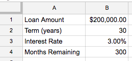
The examples below will rely on a few pieces of info about the loan in question. In particular:

• The loan value (the amount borrowed)
• The “term” of the loan (how long the loan lasts for)
• The interest rate of the loan
• How many months before the loan is paid off

For the examples below, put the following pieces in your spreadsheet the same way I did:

1. What should I expect my monthly payment to be?

One of the fundamental financial formulas in Excel is the PMT function, which tells you the total payment for a standard fixed-rate loan.

There are more complex versions of this, but we can do with the simple one:

=-PMT(rate, number_of_periods, present_value)

As straightforward as this might seem, there’s a bit of nuance to how to use this:

• rate should be our annual rate divided by 12 (3%/12); interest is typically compounded monthly, so we divide the rate by 12 to figure out what the monthly rate is
• number_of_periods should be whatever our term length is in years multiplied by 12; again interest is compounded monthly, so we have 30*12 = 360 periods
• present_value is the total loan amount ($200k)
• Note that there’s a negative sign up front; this is just to make the number look prettier. Based on accounting terminology, the payment shows up as a negative number when you use the formula. Put a negative sign up front and you should be happier.

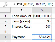
So for our sheet, this is the formula that will tell us our loan payment:

=-PMT(B3/12, B2*12, B1)

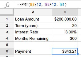
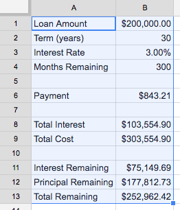
On a $200,000 loan for 30 years at 3%, the monthly payment should be $843.21.

Now that we’ve got a payment calculator all set up for you, go ahead and plug in your own mortgage or student loan values if you’ve got one. Make sure to use the initial loan value (not what you’ve got left to pay off); whatever you see there should line up with your monthly payment.

Note: for a mortgage, this payment number doesn’t include what your bank might withhold for escrow (the money they save for you to cover homeowner’s insurance and property tax costs)

Well done - no more googling “loan payment calculator” for you, young grasshopper - you just completed the first level of Spreadsheet Fu.

2. How much total interest am I going to pay on my loan?

Excel has a perfect function for this question - the CUMIPMT function.

This function calculates “cumulative interest payments” over a portion (or all of) a loan with just a few pieces of info:

=-CUMIPMT(rate, number_of_periods, present_value, first_period, last_period, end_or_beginning)

For this formula, rate, number_of_periods, and present_value are the same as the payment example above. For the others:

• first_period should be 1 and last_period should be 12*30 (360) - this is just saying we want to add the interest starting from the very first payment to the very last payment
• end_or_beginning should be 0; when this is 0 it means that payments are due at the end of each period, which is how a normal mortgage functions
• Note that there’s the negative number thing again. Same deal as before

With all of this, we can put this formula in our spreadsheet to get a “total interest payment calculator”

=-CUMIPMT(B1/12, B2*12, B3, 1, B2*12, 0)

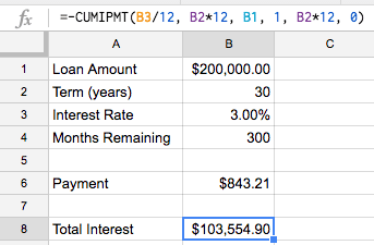
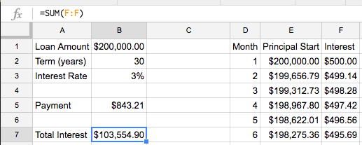
On a $200,000 loan for 30 years at 3%, the total cost of interest is $103,554.90. That’s right; even with surprisingly low interest rates, a 30-year loan can still cost you an extra 50% of your loan value in interest

3. Wait, how much am I really paying back in total?

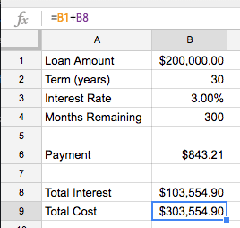
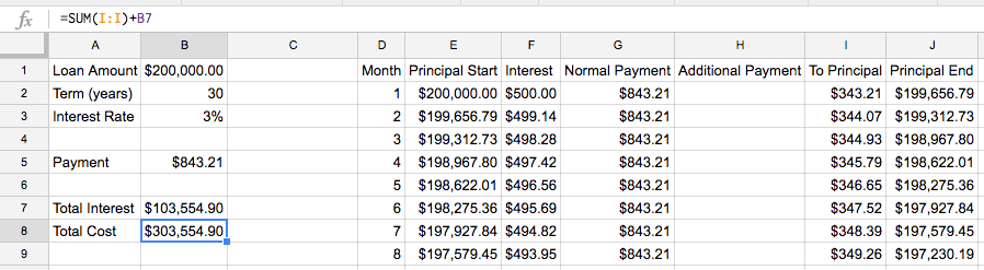
All you need to do here is to add the “Total Interest” amount to the “Loan Amount” and you’ll get a picture of what the total cost is. For our mortgage example, the $200k loan quickly turned into over $300k once the interest gets added in:

=B1+B8

4. Ok, what’s done is done - how much interest and principal do I have to go from here?

As you may have guessed, the CUMIPMT function has a counterpart - the CUMPRINC function, which calculates the cumulative principal payment over a portion (or all of) a loan.

=-CUMPRINC(rate, number_of_periods, present_value, first_period, last_period, end_or_beginning)

Look familiar? That’s right, it takes the same inputs as CUMIPMT so life is pretty easy. If we wanted to see the cumulative principal payment for our loan, we’d use the same inputs as we did for the interest formula but just use CUMPRINC instead.

That said, the answer is pretty boring:

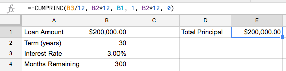
Whoop-de-doo; we proved that you have to pay $200k in principal on a $200k loan.

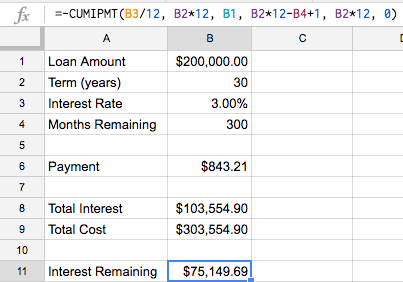
What does get interesting though is when we use CUMIPMT and CUMPRINC to understand how much is left on a loan that’s already partway paid off.

We’re finally going to use the last of our inputs - the “Months Remaining” number we put in cell B4

We want to take advantage of the first period and last period inputs to each of our cumulative payment functions.

• last period should be 360; the last month of the loan (or to keep our spreadsheet flexible, we’ll do B2*12)
• first period is a bit more complex: B2*12-B4+1; with a 360 month loan and 300 months left, we want to start looking at month 61 (360 - 300 + 1). If we had 1 month left, we’d want to look just at month 360 (360 - 360 + 1) and if we had 360 months left, we’d want to start looking at month 1 (360 - 360 + 1).

Putting this in for both CUMIPMT and CUMPRINC, we get

=-CUMIPMT(B3/12, B2*12, B1, B2*12-B4+1, B2*12, 0)

and

=-CUMPRINC(B3/12,B2*12,B1,B2*12-B4+1,B2*12,0)

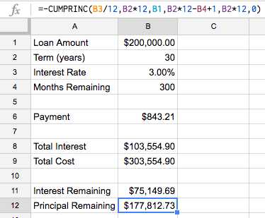
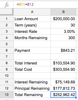
Adding the two together, we get:

=B11+B12

5. Maybe I want to refinance; is that a good idea?

Here’s where you can start informing the “what if” scenarios in your head. Let’s use Excel to analyze refinancing the loan to see what the pros and cons are.

First, highlight everything we’ve put in so far - we want to copy our progress but re-typing everything is too much work.

Once you’ve got everything highlighted, then copy (ctrl-c on Windows; command-c on Mac) the contents. Navigate to cell D1 and paste (ctrl-v on Windows; command-v on Mac)

Now you’ve duplicated the formulas and we can do a side-by-side comparison. Let’s keep the current loan in columns A and B and put the new loan in columns D and E

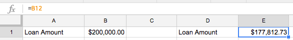
To analyze a refinance, you want to make the new loan amount (E1) equal to the current remaining principal (B12)

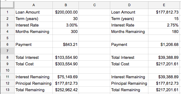
Once you’ve got this, enter in the terms of the new loan. Let’s say it’s a 15-year at 2.75%; this gives us 180 months remaining since we’re starting from scratch with a new loan.

By just plugging in the new numbers we can put the scenarios side-by-side and see the difference:

We can even add some helper formulas to make the comparison easier

• Total savings from refinancing =B13-E13
• Total increase in payment =E6-B6

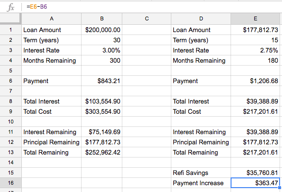
In our $200k loan example, refinancing to a 15-year at 2.75% would increase our monthly payment by $363.47 but save us $35,760.81 in interest and we’d be done 120 months (10 years) earlier.

Now we’ve got payments, interest, and refinancing down - you’ve completed level 2 of Spreadsheet Fu. Well done! Are you ready for the next challenge? This one’s big but when you’re done you’ll be ready to give your debt a thrashing.

6. What kind of impact would prepayments make?

The formulas above are great if you’re only ever going to make normal payments - they aren’t built to allow prepayment math.

That said, normal payments give you normal results. Prepayments give you awesome results :)

We can still use spreadsheets to model prepayments, it just takes a bit more work, but I promise it’s worth it. In this case, we’re actually going to build a full, flexible amortization table.

If you’re not familiar with an amortization table, it’s just a table that shows what happens to your mortgage each month - the amount you pay, the portion that goes to interest, and how much you still owe on the loan at the end of the month.

If you can put together an amortization table, you can model just about any scenario of prepayment for your loan and get a good understanding of their impact.

Lets get started with a new sheet.

Step 1 - Entering the loan inputs

Start by putting in the basic loan information; we’l use the same assumptions as we have for the other examples:

Step 2 - Structure the table

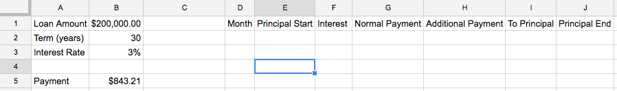
Next, we’ll set up the structure of the table by labeling the columns we intend to fill:

• Month will simply be an indicator of what month we’re looking at of the loan. Sometimes I’ll leave this purely numerical (1, 2, 3, …); others I’ll show by date (August 2016, September 2016, …).
• Principal Start will be the amount of principal remaining on the loan at the start of the month (before that month’s payment is applied)
• Interest will be the amount of interest charged on the loan that month
• Normal Payment will be the expected loan payment amount (the amount we get from using the PMT function)
• Additional Payment will be any money applied to the loan beyond the Normal Payment - this could be a one-time pay-down or a recurring monthly “extra payment”
• To Principal will be the amount of money from the Normal Payment and Additional Payment that gets applied to paying down the principal on the loan (as opposed to what goes to paying the interest)
• Principal End will be the amount of principal remaining on the loan at the end of the month (after that month’s payment is applied)

I’ll give details in the steps below on how to write the formulas for each of these. In the meantime, let’s just put the headings on columns D through J

Step 3 - Set up month one

Now we’re ready to get started with the formulas. First let’s fill in month one.

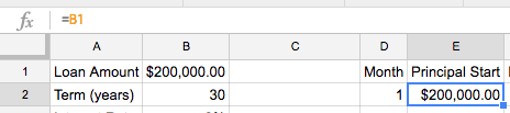
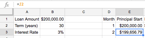
Put a 1 in cell D2 to indicate we’re looking at month one.

Next, use the loan amount in B2 as our Principal Start in E2

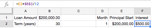
The Interest calculation is fairly simple - multiply the Principal Start by the interest rate divided by 12 (once again, we divide the interest rate by 12 to convert the annual interest rate into the monthly rate).

=E2*$B$3/12

If you’re not sure what the $ signs are for in the formula, check out this primer on Relative vs Absolute References in Excel

For the Normal Payment, we’ll just link to what we’ve got in B5 (using $B$5 as an absolute reference so we don’t lose the link to the cell when we fill in the rest of our table)

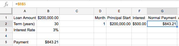
For now, let’s assume no prepayment, so we’ll leave Additional Payment blank.

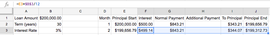
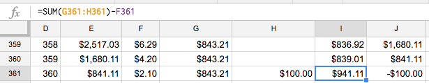
We’ll still set up the sheet to handle additional payments for later though, so our Contribution to Principal will be our Normal Payment plus our Additional Payment minus the amount of the payment applied to Interest

=SUM(G2:H2)-F2

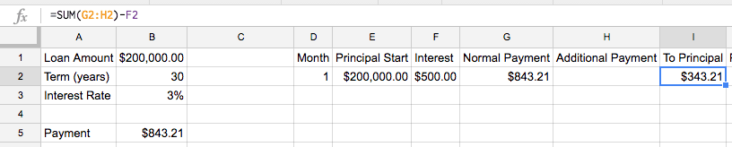
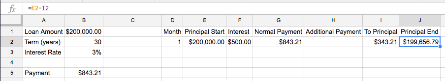
We can then subtract the Contribution to Principal from our Principal Start to get Principal End

=E2-I2

Awesome - you’ve got month one all set up.

Step 4 - Set up month two

Next we’ll fill out month two. Before you get worried, no I’m not going to do one month at a time for all 360 months of a 30-year loan.

By structuring our formulas right, all we have to do now is fill in month two and then copy and paste for the rest of the months to get our data filled in.

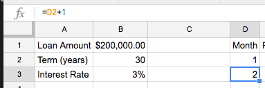
First, we’ll dynamically fill in the Month by adding 1 to the value in the month cell above the one we’re looking at. Since we’re in D3, this gives us a month formula of:

=D2+1

Principal Start in this month is simply equal to the Principal End from the last month (=J2)

For the other formulas, highlight cells F2 through J2 and copy (ctrl-c for Windows, command-c for Mac) then paste (ctrl-v for Windows, command-c for Mac) them into cells F3 through J3

Because of the way we wrote the absolute references and relative references in our formulas, we’ve made filling in month two easy and now filling in the rest of the table is even easier

Step 5 - Fill the rest of the table

Now we can use the formulas for Month two (D3 through J3) to fill in the rest of the table.

First, highlight D3 through J3 and copy.

Next, highlight D4 through J361 and paste.

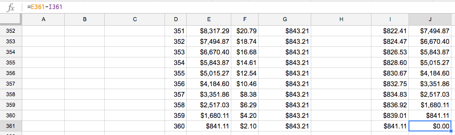
You should see the whole table fill in and ad the very end you should see a Principal End of $0.00 showing the loan paid off after 360 months.

Step 6 - Fix the table to handle a non-standard normal payment at the end of the loan

We’re in pretty good shape but our table isn’t quite set up to handle prepayments perfectly. Let’s take a look at the first problem.

Go to cell H360 (the Additional Payment cell for month 359) and enter $100. Notice an issue?

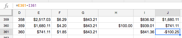
Our Principal End in month 360 now shows a negative balance, meaning we “overpaid” the loan. Obviously that’s not right so we need to find some way to fix this.

The core of this issue comes from the fact that we still applied a Normal Payment in month 360 even though the Principal Start was less than our Normal Payment.

Let’s tweak the Normal Payment formula to fix this. Edit the formula in G361:

=MIN($B$5, E361+F361)

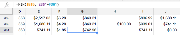
This makes sure that the Normal Payment will never exceed the remaining principal (with new interest included) by choosing the smaller of that value or the Normal Payment

Now that we’ve fixed it for month 360, fix it for the rest of the table by copying G361 and pasting for the range of cells from G2 to G361

Step 7 - Fix the table to prevent overpayment at the end of the loan from a prepayment

That fixed the problem of “overpaying” because of a normal payment. But what about “overpaying” because of a prepayment?

Delete the $100 out of H360 and put $100 in H361 instead.

Whoops - that’s definitely not what we wanted.

We could try to fix the same way we did in step 6 by taking the minimum of the Additional Payment or the amount remaining after the Normal Payment, but there’s a problem with that.

We expect that people will be typing directly into the Additional Payment column since we want the flexibility of looking at one-off prepayments in addition to regularly scheduled ones.

If we try to fix this by a formula in the Additional Payment column, it’ll just get blown away when we type our payment values directly in.

Instead, let’s fix this by capping the To Principal column. Fix the one in I361 first using the MIN formula:

=MIN(SUM(G361:H361)-F361, E361)

MIN simply selects the smallest value provided as an input

This ensures that the total payment toward principal doesn’t exceed the principal remaining (with new interest included).

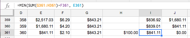
Once again, we’ve fixed this for one cell (I361) but need this across the whole table. Copy I361 and paste the formula for the whole range of I2 to I361

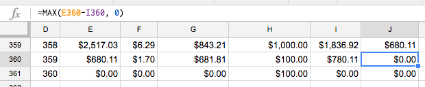
Step 8 - Fix the table to prevent a negative principal balance

You might think we’ve got everything covered, but there’s actually one more case that can trip us up - what if we end up overpaying because of both Normal Payment and Additional Payment?

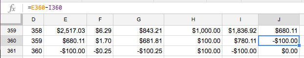
In this example, we end up overshooting in month 359 even though we adjusted for overpayment on Normal Payment and Additional Payment

At this point, we can fix this by ensuring that Principal End never goes below zero. Fixing for J360 looks like this:

=MAX(E360-I360,0)

MAX simply selects the largest value provided as an input

Once you’ve fixed this for J360, copy and paste for J2 through J361 to fix the whole table.

Now that we’ve fixed all our issues, let’s have some fun summarizing the data for ourselves so we can quickly assess how awesome our “what-if” scenarios are for prepayment.

Step 9 - Add some awesome summary data

Exciting piece of info number one is computing the Total Interest paid on a loan. As you apply prepayments, the total amount of interest you pay will go down because you’ve reduced the principal for that month and every month thereafter.

Since interest is computed on the principal remaining for each month, dropping the principal for all forward-going months has powerful effects.

Because of how we structured our table, computing the interest is fairly straightforward:

=SUM(F:F)

Column F contains all of the interest payments, so we simply sum the whole column to see what our total interest is.

Next, we can figure out the total cost of the loan (principal plus interest) by using our Total Interest result and applying the same summing principal on our To Principal column

=SUM(I:I)+B7

To test things out, let’s apply a standard Additional Payment of $100.

Enter $100 in H2 and the copy and paste through H361. If you scroll down to month 303, this is what you should see:

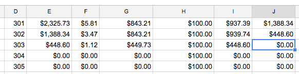
That’s right, putting an extra $100 a month to this loan means it gets paid off in month 303 (57 months early!). Not too shabby.

It’d be nice to summarize this with our other summary data though so we don’t have to scroll through the table to see how long it takes to pay off the loan in each scenario we want to run.

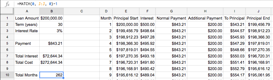
We can accomplish this using the MATCH formula:

=MATCH(0, J:J, 0)-1

MATCH looks through a range of values and returns how many values it had to look at sequentially before finding one that hit. In this case, we are looking for a value of 0 in column J that exactly matches (equals 0) and subtracting 1 because we don’t want to count looking at the column heading in J1

Step 10 - Play with the scenarios and marvel at your awesomeness

You can exhale - that’s it! Our table is all set up so now we’re ready for the fun part - playing with the different scenarios.

Looking above, a prepayment of $100 a month for the duration of the loan helps you finish the loan 57 months early and saves about $28,000 in total cost.

Let’s use the sheet to see what happens with a $200 per month prepayment. Simply put $200 in H2 and paste through H361. Checking our summary data, here’s what we see:

An extra $200 a month prepayment on this loan helps you finish 98 months early and saves about $31,000 in total cost.

It took some work to get everything set up, but now we’re free to play around with any of the inputs (Loan Amount, Term (years), Interest Rate, and the Additional Payment column) to see what the world looks like with different loans and payment strategies.

Try plugging numbers in for a loan you have - see what putting a prepayment in (start with whatever next month would be in the loan) and see how it all plays out!

After all that, you’re easily on level 3 of Spreadsheet Fu. You’re well set up to understand the fundamentals of loans and to get answers for yourself on how to best tackle them.

Go out and apply that knowledge!

Knowing is not enough, we must apply. Willing is not enough, we must do

Bruce Lee

Want to become a Spreadsheet black belt? Subscribe to my email list below to make sure you don’t miss future posts and opportunities to learn more!